Decision Trees

Decision Trees (DTs) are a supervised learning algorithm that learns simple decision rules, to assign predictions to. Example: If age < 30 and income > 50,000 then: "Rich", else: "Not Rich".

Advantages of Decision Trees

Firslty, they can do both Regression and Classification tasks.

Secondly, “White Box”: Simple to understand and to interpret. This is their fundamental advantage. You do not get this level of interpretability with Deep Neural Networks (a “Black Box”)

You can map the exact sequence of logical conditions the algorithm evaluated to reach a conclusion. If a medical triage model recommends prescribing antibiotics, you can trace the decision branches back to see exactly why (e.g., "Body Temperature > 38°C" AND "Rapid Strep Test = Positive").

Trees can also be visualized.

Thirdlay, they can handle Multi-output problems.

Fourthly, inference cost is logarithmic in the number of data points used to train the tree. That means even if your dataset is massive, the time it takes to make a prediction barely increases.

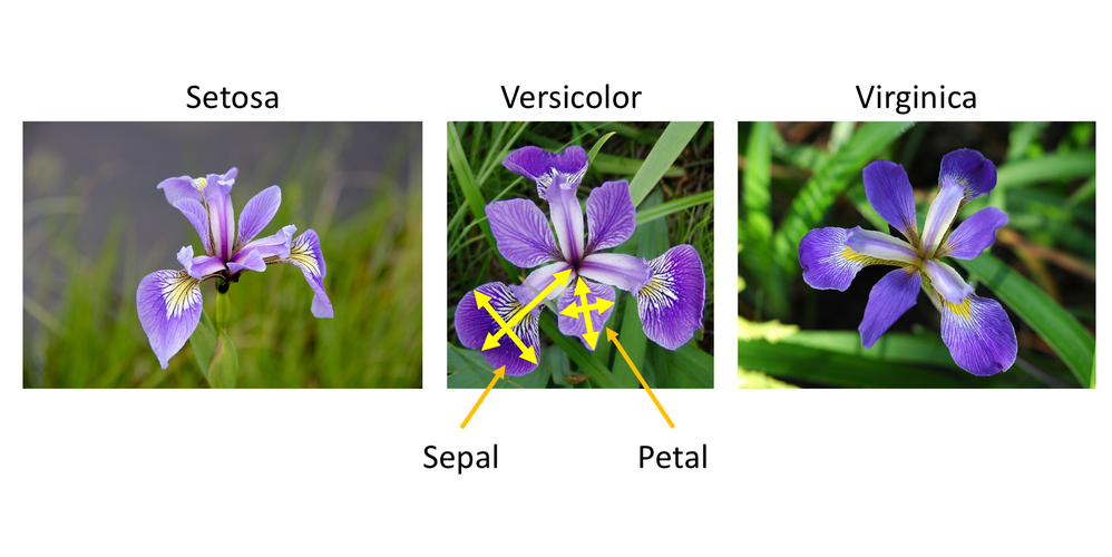
Example: Iris Flowers Classification

For instance, in the example below, decision trees learn from data to approximate a sine curve with a set of if-then-else decision rules. The deeper the tree, the more complex the decision rules and the fitter the model.

from sklearn.datasets import load_iris

iris = load_iris(as_frame=True)
X, y = iris.data, iris.target

import pandas as pd

pd.concat([iris.data, iris.target], axis=1)

	sepal length (cm)	sepal width (cm)	petal length (cm)	petal width (cm)	target
0	5.1	3.5	1.4	0.2	0
1	4.9	3.0	1.4	0.2	0
2	4.7	3.2	1.3	0.2	0
3	4.6	3.1	1.5	0.2	0
4	5.0	3.6	1.4	0.2	0
...	...	...	...	...	...
145	6.7	3.0	5.2	2.3	2
146	6.3	2.5	5.0	1.9	2
147	6.5	3.0	5.2	2.0	2
148	6.2	3.4	5.4	2.3	2
149	5.9	3.0	5.1	1.8	2

150 rows × 5 columns

from sklearn.tree import DecisionTreeClassifier

X_iris = iris.data[["petal length (cm)", "petal width (cm)"]].values
y_iris = iris.target

tree_clf = DecisionTreeClassifier(max_depth=2, random_state=42)
tree_clf.fit(X_iris, y_iris)

DecisionTreeClassifier(max_depth=2, random_state=42)

In a Jupyter environment, please rerun this cell to show the HTML representation or trust the notebook.
On GitHub, the HTML representation is unable to render, please try loading this page with nbviewer.org.

After being fitted, the model can then be used to predict the class of samples:

tree_clf.predict([[5.1, 3.5]])

array([2])

The probability of each class can be predicted, which is: the fraction of training samples of the class in a leaf:

tree_clf.predict_proba([[5.1, 3.5]]).round(3)

array([[0.   , 0.022, 0.978]])

الكود

from sklearn.tree import plot_tree
import matplotlib.pyplot as plt

plt.figure(figsize=(18, 10))
plot_tree(
    tree_clf, 
    feature_names=iris.feature_names, 
    class_names=iris.target_names, 
    filled=True, 
    rounded=True, 
    fontsize=12,
    proportion=False,
    impurity=False # Hides impurity to reduce clutter
)
plt.title("Decision Tree for Iris Dataset", fontsize=16)
plt.show()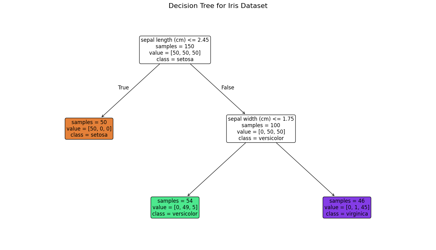

الكود

import numpy as np
import matplotlib.pyplot as plt

# extra code – just formatting details
from matplotlib.colors import ListedColormap
custom_cmap = ListedColormap(['#fafab0', '#9898ff', '#a0faa0'])
plt.figure(figsize=(8, 4))

lengths, widths = np.meshgrid(np.linspace(0, 7.2, 100), np.linspace(0, 3, 100))
X_iris_all = np.c_[lengths.ravel(), widths.ravel()]
y_pred = tree_clf.predict(X_iris_all).reshape(lengths.shape)
plt.contourf(lengths, widths, y_pred, alpha=0.3, cmap=custom_cmap)
for idx, (name, style) in enumerate(zip(iris.target_names, ("yo", "bs", "g^"))):
    plt.plot(X_iris[:, 0][y_iris == idx], X_iris[:, 1][y_iris == idx],
             style, label=f"Iris {name}")

# extra code – this section beautifies and saves Figure 6–2
tree_clf_deeper = DecisionTreeClassifier(max_depth=3, random_state=42)
tree_clf_deeper.fit(X_iris, y_iris)
th0, th1, th2a, th2b = tree_clf_deeper.tree_.threshold[[0, 2, 3, 6]]
plt.xlabel("Petal length (cm)")
plt.ylabel("Petal width (cm)")
plt.plot([th0, th0], [0, 3], "k-", linewidth=2)
plt.plot([th0, 7.2], [th1, th1], "k--", linewidth=2)
plt.plot([th2a, th2a], [0, th1], "k:", linewidth=2)
plt.plot([th2b, th2b], [th1, 3], "k:", linewidth=2)
plt.text(th0 - 0.05, 1.0, "Depth=0", horizontalalignment="right", fontsize=15)
plt.text(3.2, th1 + 0.02, "Depth=1", verticalalignment="bottom", fontsize=13)
plt.text(th2a + 0.05, 0.5, "(Depth=2)", fontsize=11)
plt.axis([0, 7.2, 0, 3])
plt.legend()

plt.show()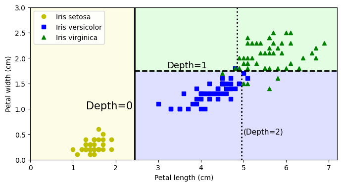

Avoid Overfitting

Decision trees tend to overfit on data with a small samples-to-features ratio. A decision tree will keep growing branches until it has a specific rule for every single data point.

In scikit-learn, restricting a decision tree so it doesn’t memorize your training data is known as regularization or pruning.

If you are just starting out, adjusting max_depth and min_samples_leaf will give you the most immediate control over overfitting.

Let’s illustrate the problem:

from sklearn.datasets import make_moons

X_moons, y_moons = make_moons(n_samples=150, noise=0.2, random_state=42)

tree_clf1 = DecisionTreeClassifier(random_state=42)
tree_clf2 = DecisionTreeClassifier(min_samples_leaf=5, random_state=42)
tree_clf1.fit(X_moons, y_moons)
tree_clf2.fit(X_moons, y_moons)

DecisionTreeClassifier(min_samples_leaf=5, random_state=42)

الكود

def plot_decision_boundary(clf, X, y, axes, cmap):
    x1, x2 = np.meshgrid(np.linspace(axes[0], axes[1], 100),
                         np.linspace(axes[2], axes[3], 100))
    X_new = np.c_[x1.ravel(), x2.ravel()]
    y_pred = clf.predict(X_new).reshape(x1.shape)
    
    plt.contourf(x1, x2, y_pred, alpha=0.3, cmap=cmap)
    plt.contour(x1, x2, y_pred, cmap="Greys", alpha=0.8)
    colors = {"Wistia": ["#78785c", "#c47b27"], "Pastel1": ["red", "blue"]}
    markers = ("o", "^")
    for idx in (0, 1):
        plt.plot(X[:, 0][y == idx], X[:, 1][y == idx],
                 color=colors[cmap][idx], marker=markers[idx], linestyle="none")
    plt.axis(axes)
    plt.xlabel(r"$x_1$")
    plt.ylabel(r"$x_2$", rotation=0)

fig, axes = plt.subplots(ncols=2, figsize=(10, 4), sharey=True)
plt.sca(axes[0])
plot_decision_boundary(tree_clf1, X_moons, y_moons,
                       axes=[-1.5, 2.4, -1, 1.5], cmap="Wistia")
plt.title("No restrictions")
plt.sca(axes[1])
plot_decision_boundary(tree_clf2, X_moons, y_moons,
                       axes=[-1.5, 2.4, -1, 1.5], cmap="Wistia")
plt.title(f"min_samples_leaf = {tree_clf2.min_samples_leaf}")
plt.ylabel("")
plt.show();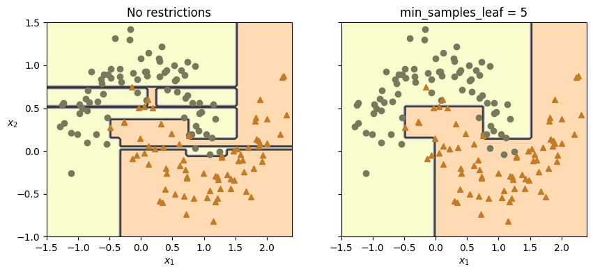

X_moons_test, y_moons_test = make_moons(
    n_samples=1000,
    noise=0.2,
    random_state=43
)

print(tree_clf1.score(X_moons_test, y_moons_test))
print(tree_clf2.score(X_moons_test, y_moons_test))

0.898
0.92

1. The Manual Approach: Setting Limits Directly

from sklearn.tree import DecisionTreeClassifier

# Create the tree and set your boundaries right from the start
# We cap the tree at 5 questions deep and force at least 10 data points per final leaf.
my_tree = DecisionTreeClassifier(
    max_depth=5,
    min_samples_leaf=10
)

# Train the model on your data (X contains your data, y contains the answers)
# my_tree.fit(X, y)

2. The Automated Approach: Grid Search

from sklearn.tree import DecisionTreeClassifier
from sklearn.model_selection import GridSearchCV

# 1. Create a blank tree with no rules yet
blank_tree = DecisionTreeClassifier()

# 2. Create your "menu" of options to test (this is your grid)
options_to_test = {
    'max_depth': [3, 5, 7, 10, None],  # Test shallow, medium, deep, and unrestricted
    'min_samples_leaf': [2, 5, 10, 20] # Test different bucket sizes
}

# 3. Set up the automated tester
# cv=5 means "Cross-Validation". It tests every combination 5 separate times 
# on different slices of your data to ensure the results aren't just a lucky fluke.
automated_tester = GridSearchCV(
    estimator=blank_tree,
    param_grid=options_to_test,
    cv=5
)

# 4. Start the test (this might take a moment depending on how big your data and menu are)
# automated_tester.fit(X, y)

# 5. Print out the winning combination!
# print("The best limits to use are:", automated_tester.best_params_)

Here is the full list of the hyperparameters you can set to stop this from happening, broken down by how they control the tree:

1. Controlling the Architecture (Pre-pruning)

These parameters stop the tree from growing too large in the first place.

`max_depth`

What it does: Sets a hard limit on how many levels (or questions) deep the tree can go.
How it helps: By changing this from its default (None) to a specific number (like 3, 5, or 10), you force the algorithm to stop drilling down into hyper-specific patterns. It keeps the model focused on the broad, general rules.

`min_samples_split`

What it does: Dictates the minimum number of data points a branch must have before it is allowed to split again.
How it helps: If you set this to 20, any “bucket” of data containing 19 or fewer samples will refuse to split further. This stops the tree from creating complex rules just to satisfy a tiny handful of data points.

`min_samples_leaf`

What it does: Dictates the minimum number of data points that must end up in a final leaf node after a split.
How it helps: A split will only be allowed if both the resulting left and right branches contain at least this many samples. This is highly effective at preventing the tree from isolating random outliers into their own custom leaves.

`max_leaf_nodes`

What it does: Caps the total number of endpoints the tree is allowed to have.
How it helps: If set to 15, the algorithm will find the 15 most important splits (the ones that reduce the most error) and then strictly stop.

2. Introducing Randomness

`max_features`

What it does: Limits how many variables (columns) the algorithm is allowed to look at when deciding how to split a node.
How it helps: If you have 20 variables, you can tell the tree to only consider a random subset of 5 variables at every split. This forces the tree to look for alternative patterns and prevents it from becoming overly dependent on just one dominant variable.

3. Mathematical Pruning (Post-pruning)

`ccp_alpha` (Cost-Complexity Pruning)

What it does: It allows the tree to grow fully, but then mathematically calculates the “cost” of each branch. It penalizes branches that are overly complex but don’t add much predictive value.
How it helps: Increasing this number acts like a pair of hedge clippers. A higher ccp_alpha snips off weak branches from the bottom up, leaving you with a simpler, more robust tree.

See Example: Post pruning decision trees with cost complexity pruning.

Learn more Tips on Practical Use.

References: https://github.com/ageron/handson-ml3/blob/main/06_decision_trees.ipynb

	criterion criterion: {"gini", "entropy", "log_loss"}, default="gini" The function to measure the quality of a split. Supported criteria are "gini" for the Gini impurity and "log_loss" and "entropy" both for the Shannon information gain, see :ref:`tree_mathematical_formulation`.	'gini'
	splitter splitter: {"best", "random"}, default="best" The strategy used to choose the split at each node. Supported strategies are "best" to choose the best split and "random" to choose the best random split.	'best'
	max_depth max_depth: int, default=None The maximum depth of the tree. If None, then nodes are expanded until all leaves are pure or until all leaves contain less than min_samples_split samples.	2
	min_samples_split min_samples_split: int or float, default=2 The minimum number of samples required to split an internal node: - If int, then consider `min_samples_split` as the minimum number. - If float, then `min_samples_split` is a fraction and `ceil(min_samples_split * n_samples)` are the minimum number of samples for each split. .. versionchanged:: 0.18 Added float values for fractions.	2
	min_samples_leaf min_samples_leaf: int or float, default=1 The minimum number of samples required to be at a leaf node. A split point at any depth will only be considered if it leaves at least ``min_samples_leaf`` training samples in each of the left and right branches. This may have the effect of smoothing the model, especially in regression. - If int, then consider `min_samples_leaf` as the minimum number. - If float, then `min_samples_leaf` is a fraction and `ceil(min_samples_leaf * n_samples)` are the minimum number of samples for each node. .. versionchanged:: 0.18 Added float values for fractions.	1
	min_weight_fraction_leaf min_weight_fraction_leaf: float, default=0.0 The minimum weighted fraction of the sum total of weights (of all the input samples) required to be at a leaf node. Samples have equal weight when sample_weight is not provided.	0.0
	max_features max_features: int, float or {"sqrt", "log2"}, default=None The number of features to consider when looking for the best split: - If int, then consider `max_features` features at each split. - If float, then `max_features` is a fraction and `max(1, int(max_features * n_features_in_))` features are considered at each split. - If "sqrt", then `max_features=sqrt(n_features)`. - If "log2", then `max_features=log2(n_features)`. - If None, then `max_features=n_features`. .. note:: The search for a split does not stop until at least one valid partition of the node samples is found, even if it requires to effectively inspect more than ``max_features`` features.	None
	random_state random_state: int, RandomState instance or None, default=None Controls the randomness of the estimator. The features are always randomly permuted at each split, even if ``splitter`` is set to ``"best"``. When ``max_features < n_features``, the algorithm will select ``max_features`` at random at each split before finding the best split among them. But the best found split may vary across different runs, even if ``max_features=n_features``. That is the case, if the improvement of the criterion is identical for several splits and one split has to be selected at random. To obtain a deterministic behaviour during fitting, ``random_state`` has to be fixed to an integer. See :term:`Glossary ` for details.	42
	max_leaf_nodes max_leaf_nodes: int, default=None Grow a tree with ``max_leaf_nodes`` in best-first fashion. Best nodes are defined as relative reduction in impurity. If None then unlimited number of leaf nodes.	None
	min_impurity_decrease min_impurity_decrease: float, default=0.0 A node will be split if this split induces a decrease of the impurity greater than or equal to this value. The weighted impurity decrease equation is the following:: N_t / N * (impurity - N_t_R / N_t * right_impurity - N_t_L / N_t * left_impurity) where ``N`` is the total number of samples, ``N_t`` is the number of samples at the current node, ``N_t_L`` is the number of samples in the left child, and ``N_t_R`` is the number of samples in the right child. ``N``, ``N_t``, ``N_t_R`` and ``N_t_L`` all refer to the weighted sum, if ``sample_weight`` is passed. .. versionadded:: 0.19	0.0
	class_weight class_weight: dict, list of dict or "balanced", default=None Weights associated with classes in the form ``{class_label: weight}``. If None, all classes are supposed to have weight one. For multi-output problems, a list of dicts can be provided in the same order as the columns of y. Note that for multioutput (including multilabel) weights should be defined for each class of every column in its own dict. For example, for four-class multilabel classification weights should be [{0: 1, 1: 1}, {0: 1, 1: 5}, {0: 1, 1: 1}, {0: 1, 1: 1}] instead of [{1:1}, {2:5}, {3:1}, {4:1}]. The "balanced" mode uses the values of y to automatically adjust weights inversely proportional to class frequencies in the input data as ``n_samples / (n_classes * np.bincount(y))`` For multi-output, the weights of each column of y will be multiplied. Note that these weights will be multiplied with sample_weight (passed through the fit method) if sample_weight is specified.	None
	ccp_alpha ccp_alpha: non-negative float, default=0.0 Complexity parameter used for Minimal Cost-Complexity Pruning. The subtree with the largest cost complexity that is smaller than ``ccp_alpha`` will be chosen. By default, no pruning is performed. See :ref:`minimal_cost_complexity_pruning` for details. See :ref:`sphx_glr_auto_examples_tree_plot_cost_complexity_pruning.py` for an example of such pruning. .. versionadded:: 0.22	0.0
	monotonic_cst monotonic_cst: array-like of int of shape (n_features), default=None Indicates the monotonicity constraint to enforce on each feature. - 1: monotonic increase - 0: no constraint - -1: monotonic decrease If monotonic_cst is None, no constraints are applied. Monotonicity constraints are not supported for: - multiclass classifications (i.e. when `n_classes > 2`), - multioutput classifications (i.e. when `n_outputs_ > 1`), - classifications trained on data with missing values. The constraints hold over the probability of the positive class. Read more in the :ref:`User Guide `. .. versionadded:: 1.4	None

	criterion criterion: {"gini", "entropy", "log_loss"}, default="gini" The function to measure the quality of a split. Supported criteria are "gini" for the Gini impurity and "log_loss" and "entropy" both for the Shannon information gain, see :ref:`tree_mathematical_formulation`.	'gini'
	splitter splitter: {"best", "random"}, default="best" The strategy used to choose the split at each node. Supported strategies are "best" to choose the best split and "random" to choose the best random split.	'best'
	max_depth max_depth: int, default=None The maximum depth of the tree. If None, then nodes are expanded until all leaves are pure or until all leaves contain less than min_samples_split samples.	None
	min_samples_split min_samples_split: int or float, default=2 The minimum number of samples required to split an internal node: - If int, then consider `min_samples_split` as the minimum number. - If float, then `min_samples_split` is a fraction and `ceil(min_samples_split * n_samples)` are the minimum number of samples for each split. .. versionchanged:: 0.18 Added float values for fractions.	2
	min_samples_leaf min_samples_leaf: int or float, default=1 The minimum number of samples required to be at a leaf node. A split point at any depth will only be considered if it leaves at least ``min_samples_leaf`` training samples in each of the left and right branches. This may have the effect of smoothing the model, especially in regression. - If int, then consider `min_samples_leaf` as the minimum number. - If float, then `min_samples_leaf` is a fraction and `ceil(min_samples_leaf * n_samples)` are the minimum number of samples for each node. .. versionchanged:: 0.18 Added float values for fractions.	5
	min_weight_fraction_leaf min_weight_fraction_leaf: float, default=0.0 The minimum weighted fraction of the sum total of weights (of all the input samples) required to be at a leaf node. Samples have equal weight when sample_weight is not provided.	0.0
	max_features max_features: int, float or {"sqrt", "log2"}, default=None The number of features to consider when looking for the best split: - If int, then consider `max_features` features at each split. - If float, then `max_features` is a fraction and `max(1, int(max_features * n_features_in_))` features are considered at each split. - If "sqrt", then `max_features=sqrt(n_features)`. - If "log2", then `max_features=log2(n_features)`. - If None, then `max_features=n_features`. .. note:: The search for a split does not stop until at least one valid partition of the node samples is found, even if it requires to effectively inspect more than ``max_features`` features.	None
	random_state random_state: int, RandomState instance or None, default=None Controls the randomness of the estimator. The features are always randomly permuted at each split, even if ``splitter`` is set to ``"best"``. When ``max_features < n_features``, the algorithm will select ``max_features`` at random at each split before finding the best split among them. But the best found split may vary across different runs, even if ``max_features=n_features``. That is the case, if the improvement of the criterion is identical for several splits and one split has to be selected at random. To obtain a deterministic behaviour during fitting, ``random_state`` has to be fixed to an integer. See :term:`Glossary ` for details.	42
	max_leaf_nodes max_leaf_nodes: int, default=None Grow a tree with ``max_leaf_nodes`` in best-first fashion. Best nodes are defined as relative reduction in impurity. If None then unlimited number of leaf nodes.	None
	min_impurity_decrease min_impurity_decrease: float, default=0.0 A node will be split if this split induces a decrease of the impurity greater than or equal to this value. The weighted impurity decrease equation is the following:: N_t / N * (impurity - N_t_R / N_t * right_impurity - N_t_L / N_t * left_impurity) where ``N`` is the total number of samples, ``N_t`` is the number of samples at the current node, ``N_t_L`` is the number of samples in the left child, and ``N_t_R`` is the number of samples in the right child. ``N``, ``N_t``, ``N_t_R`` and ``N_t_L`` all refer to the weighted sum, if ``sample_weight`` is passed. .. versionadded:: 0.19	0.0
	class_weight class_weight: dict, list of dict or "balanced", default=None Weights associated with classes in the form ``{class_label: weight}``. If None, all classes are supposed to have weight one. For multi-output problems, a list of dicts can be provided in the same order as the columns of y. Note that for multioutput (including multilabel) weights should be defined for each class of every column in its own dict. For example, for four-class multilabel classification weights should be [{0: 1, 1: 1}, {0: 1, 1: 5}, {0: 1, 1: 1}, {0: 1, 1: 1}] instead of [{1:1}, {2:5}, {3:1}, {4:1}]. The "balanced" mode uses the values of y to automatically adjust weights inversely proportional to class frequencies in the input data as ``n_samples / (n_classes * np.bincount(y))`` For multi-output, the weights of each column of y will be multiplied. Note that these weights will be multiplied with sample_weight (passed through the fit method) if sample_weight is specified.	None
	ccp_alpha ccp_alpha: non-negative float, default=0.0 Complexity parameter used for Minimal Cost-Complexity Pruning. The subtree with the largest cost complexity that is smaller than ``ccp_alpha`` will be chosen. By default, no pruning is performed. See :ref:`minimal_cost_complexity_pruning` for details. See :ref:`sphx_glr_auto_examples_tree_plot_cost_complexity_pruning.py` for an example of such pruning. .. versionadded:: 0.22	0.0
	monotonic_cst monotonic_cst: array-like of int of shape (n_features), default=None Indicates the monotonicity constraint to enforce on each feature. - 1: monotonic increase - 0: no constraint - -1: monotonic decrease If monotonic_cst is None, no constraints are applied. Monotonicity constraints are not supported for: - multiclass classifications (i.e. when `n_classes > 2`), - multioutput classifications (i.e. when `n_outputs_ > 1`), - classifications trained on data with missing values. The constraints hold over the probability of the positive class. Read more in the :ref:`User Guide `. .. versionadded:: 1.4	None

Advantages of Decision Trees

Example: Iris Flowers Classification

Avoid Overfitting

1. The Manual Approach: Setting Limits Directly

2. The Automated Approach: Grid Search

1. Controlling the Architecture (Pre-pruning)

max_depth

min_samples_split

min_samples_leaf

max_leaf_nodes

2. Introducing Randomness

max_features

3. Mathematical Pruning (Post-pruning)

ccp_alpha (Cost-Complexity Pruning)

`max_depth`

`min_samples_split`

`min_samples_leaf`

`max_leaf_nodes`

`max_features`

`ccp_alpha` (Cost-Complexity Pruning)