Model selection and evaluation
how to assess our model’s performance?
Loss and Error: These are objective functions optimized by the machine learning algorithm during training. The primary goal of the model is to minimize this value (e.g., Mean Squared Error for regression, or Log Loss for classification) to “learn” the patterns in the data.
Metric and Score: These are human-interpretable measures used to evaluate the model’s final performance from a practical or business perspective. While the model trains by minimizing loss, we judge its overall success and compare it against other models using metrics (e.g., Accuracy, R-squared, Precision, or Recall).
In scikit-learn:
- Score: higher is better.
- Error: lower is better.
Checkout the Guide on 3.4. Metrics and scoring: quantifying the quality of predictions for practical tips on which scoring function should you use.
Take a quick peek at:
why do we have a held-out set for testing?
Splitting a dataset into training and test sets is the primary method used to estimate how a model will perform in the real world.
In scikit-learn a random split into training and test sets can be quickly computed with the train_test_split helper function. Let’s load the iris data set to fit a linear support vector machine on it:
import numpy as np
from sklearn.model_selection import train_test_split
from sklearn import datasets
from sklearn import svm

X, y = datasets.load_iris(return_X_y=True)
X.shape, y.shape
We can now quickly sample a training set while holding out 40% of the data for testing (evaluating) our classifier:
X_train, X_test, y_train, y_test = train_test_split(
    X, y, test_size=0.4, random_state=0)

X_train.shape, y_train.shape
X_test.shape, y_test.shape

clf = svm.SVC(kernel='linear', C=1).fit(X_train, y_train)
clf.score(X_test, y_test)
In machine learning, the fundamental goal is generalization: the ability of a model to make accurate predictions on new, unseen data, rather than just “memorizing” the data it has already seen.
Using the same data for both training and evaluation creates a circular dependency. It is mathematically dishonest to test a model on the same data used to build it because the model’s error rate will be optimistically biased.
A test set provides an unbiased estimate of the model’s performance (loss, accuracy, precision, etc.) on new observations.
how do we know our model is better than a guess?
When doing supervised learning, a simple sanity check consists of comparing one’s estimator against simple rules of thumb. DummyClassifier implements several such simple strategies for classification:
constantalways predicts a constant label that is provided by the user.most_frequentalways predicts the most frequent label in the training set.stratifiedgenerates random predictions by respecting the training set class distribution.
Note that with all these strategies, the predict method completely ignores the input data!
To illustrate DummyClassifier, first let’s create an imbalanced dataset:
from sklearn.datasets import load_iris
from sklearn.model_selection import train_test_split
X, y = load_iris(return_X_y=True)
y[y != 1] = -1
X_train, X_test, y_train, y_test = train_test_split(X, y, random_state=0)
Next, let’s compare the accuracy of LogisticRegression and most_frequent:
clf = LogisticRegression(C=1).fit(X_train, y_train)
clf.score(X_test, y_test)
More generally, when the accuracy of a classifier is too close to random, it probably means that something went wrong: features are not helpful, a hyperparameter is not correctly tuned, the classifier is suffering from class imbalance, etc…
DummyRegressor also implements four simple rules of thumb for regression:
meanalways predicts the mean of the training targets.medianalways predicts the median of the training targets.quantilealways predicts a user provided quantile of the training targets.constantalways predicts a constant value that is provided by the user.
In all these strategies, the predict method completely ignores the input data.
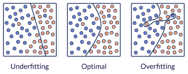
how do we avoid under-fitting and over-fitting?
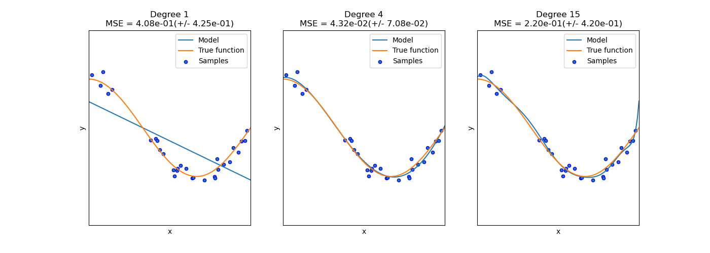
We evaluate quantitatively overfitting / underfitting by using cross-validation. We calculate the mean squared error (MSE) on the validation set, the higher, the less likely the model generalizes correctly from the training data.
Here is a flowchart of typical cross validation workflow in model training. The best parameters can be determined by grid search techniques.
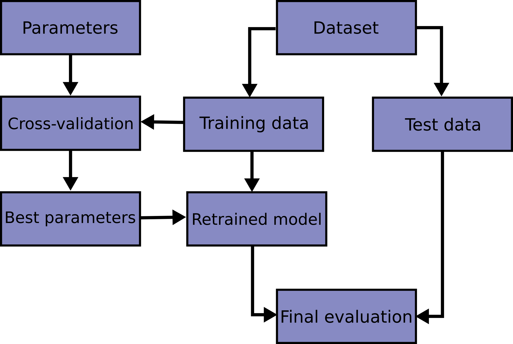
A test set should still be held out for final evaluation. In the basic approach, called k-fold CV, the training set is split into k smaller sets (other approaches generally follow the same principles). The following procedure is followed for each of the k “folds”:
- A model is trained using \(k - 1\) of the folds as training data;
- the resulting model is validated on the remaining part of the data (i.e., it is used as a test set to compute a performance measure such as accuracy).
The performance measure reported by k-fold cross-validation is then the average of the values computed in the loop.

Source: Cross-validation: evaluating estimator performance | Scikit-learn
Sometimes helpful to plot the influence of a single hyperparameter on the training score and the validation score to find out whether the estimator is overfitting or underfitting for some hyperparameter values.
from sklearn.datasets import load_iris
from sklearn.model_selection import ValidationCurveDisplay
from sklearn.svm import SVC
from sklearn.utils import shuffle
X, y = load_iris(return_X_y=True)
X, y = shuffle(X, y, random_state=0)
ValidationCurveDisplay.from_estimator(
   SVC(kernel="linear"), X, y, param_name="C", param_range=np.logspace(-7, 3, 10)
)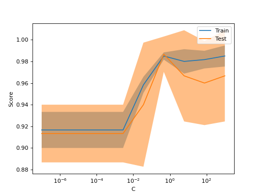
If the training score and the validation score are both low, the estimator will be underfitting. If the training score is high and the validation score is low, the estimator is overfitting and otherwise it is working very well. A low training score and a high validation score is usually not possible.
Source: 3.5.1. Validation curve.
Computing cross-validated metrics
The simplest way to use cross-validation is to call the cross_val_score helper function on the estimator and the dataset.
The following example demonstrates how to estimate the accuracy of a linear kernel support vector machine on the iris dataset by splitting the data, fitting a model and computing the score 5 consecutive times (with different splits each time):
from sklearn.model_selection import cross_val_score
clf = svm.SVC(kernel='linear', C=1, random_state=42)
scores = cross_val_score(clf, X, y, cv=5)
scores
Tuning the hyper-parameters of an estimator
How do we know to choose kernel='linear', C=1 or other hyper-parameters?
Hyper-parameters are parameters that are not directly learnt within estimators. In scikit-learn they are passed as arguments to the constructor of the estimator classes. Typical examples include C, kernel and gamma for Support Vector Classifier, alpha for Lasso, etc.
It is possible and recommended to search the hyper-parameter space for the best cross validation score.
Any parameter provided when constructing an estimator may be optimized in this manner. Specifically, to find the names and current values for all parameters for a given estimator, use:
estimator.get_params()A search consists of:
- an estimator (regressor or classifier such as
sklearn.svm.SVC());
- a parameter space;
- a search method;
- a cross-validation scheme; and
- a score function.
Hyper-parameter tuning methods
Two generic search methods:
GridSearchCVexhaustively considers all parameter combinationsRandomizedSearchCVsamples a given number of candidates from a parameter space with a specified distribution.
Note: CV stands for cross-validation.
Model-specific hyper-parameter tuning
Some models can fit data for a range of values of some parameter almost as efficiently as fitting the estimator for a single value of the parameter. This feature can be leveraged to perform a more efficient cross-validation used for model selection of this parameter.
See: 3.2.5.1. Model specific cross-validation for a list of those models.
GridSearchCV and RandomizedSearchCV allow searching over parameters of composite or nested estimators such as Pipeline, ColumnTransformer, VotingClassifier or CalibratedClassifierCV using a dedicated <estimator>__<parameter> syntax:
from sklearn.model_selection import GridSearchCV
from sklearn.calibration import CalibratedClassifierCV
from sklearn.ensemble import RandomForestClassifier
from sklearn.datasets import make_moons

X, y = make_moons()

calibrated_forest = CalibratedClassifierCV(
    estimator=RandomForestClassifier(n_estimators=10)
)

param_grid = {
   'estimator__max_depth': [2, 4, 6, 8]
}

search = GridSearchCV(
    calibrated_forest,
    param_grid,
    cv=5
)

search.fit(X, y)
Here, <estimator> is the parameter name of the nested estimator, in this case estimator. If the meta-estimator is constructed as a collection of estimators as in pipeline.Pipeline, then <estimator> refers to the name of the estimator, see Access to nested parameters. In practice, there can be several levels of nesting:
from sklearn.pipeline import Pipeline
from sklearn.feature_selection import SelectKBest

pipe = Pipeline([
   ('select', SelectKBest()),
   ('model', calibrated_forest)]
)

param_grid = {
   'select__k': [1, 2],
   'model__estimator__max_depth': [2, 4, 6, 8]
}

search = GridSearchCV(
    pipe,
    param_grid,
    cv=5
)
search.fit(X, y)
Please refer to Pipeline: chaining estimators for performing parameter searches over pipelines.
Model scalability: can we learn more?
how to answer the question: can our model learn from more data?
Learning curves show the effect of adding more samples during the training process. The effect is depicted by checking the statistical performance of the model in terms of training score and testing score.
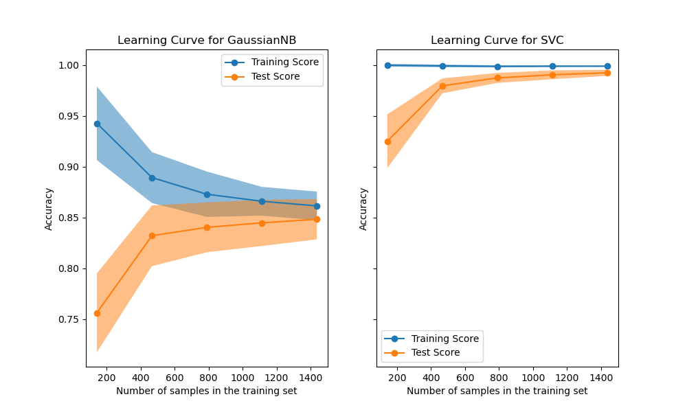
Read more: Plotting Learning Curves and Checking Models’ Scalability.
How to link models metrics to business metrics?
Classification is best divided into two parts:
- the statistical problem of learning a model to predict, ideally, class probabilities;
- the decision problem to take concrete action based on those probability predictions.
Let’s take a straightforward example related to weather forecasting: the first point is related to answering:
- “what is the chance that it will rain tomorrow?”
- “should I take an umbrella tomorrow?”
In business, we might assess impact by money loss.
Risk is the product of the probability of an event occurring and the magnitude (impact) of that event
\[Total\ Risk = \sum_{i=1}^{n} P(x_i) \cdot L(x_i)\] Where:
- \(P(E)\) is the probability of an event \(E\)
- \(L(E)\) is the loss or magnitude associated with that event
Learn more: 3.3. Tuning the decision threshold for class prediction - 3.3.1. Post-tuning the decision threshold - 3.3.1.4. Examples - See the example entitled Post-hoc tuning the cut-off point of decision function, to get insights on the post-tuning of the decision threshold. - See the example entitled Post-tuning the decision threshold for cost-sensitive learning, to learn about cost-sensitive learning and decision threshold tuning.