Module 1 - Session 2: The ML Pipeline and Building Your First Model

Session 2

The Machine Learning Pipeline

Six stages from data to deployed model

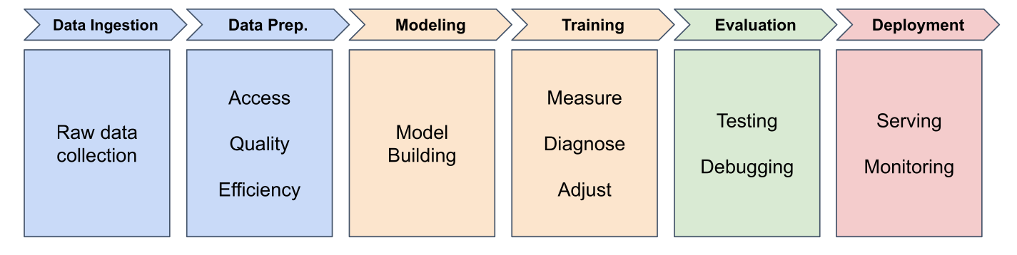
The Machine Learning Pipeline

Last session, we saw how neural networks learn using the delivery time problem. Now, before we jump into code, we need a systematic approach. This framework will be used throughout the entire Professional Certificate, whether you’re training a delivery predictor or building image classifiers later.

The pipeline ensures we don’t skip critical steps and helps us understand where we are in the process at any given time.

Stage 1: Data Ingestion

Gathering and organizing raw data

• Delivery records from company database
• Messy data: inconsistent formats, missing values, errors
• Organize for PyTorch to work efficiently

It all starts with data. Before you can train any model, you need to gather your raw information and organize it so PyTorch can work with each data point efficiently.

For the delivery predictor, that data comes from the company’s delivery records. But here’s where things get tricky - real-world data is messy. Earlier records might list delivery times as free-text entries like “22 minutes,” while newer ones use numeric values like 22.0. There are always issues: missing values, negative delivery times, or records suggesting you were biking at 200 miles per hour.

This kind of messy data is the norm, not the exception. In your first lab, we’ll keep things simple with clean data, but understanding these steps helps you appreciate what goes into real-world projects.

Stage 2: Data Preparation

Cleaning, transforming, and organizing

• Fix errors (impossible times, duplicates)
• Handle missing values
• Engineer features (addresses → distances)

Most time-consuming stage in real projects

Getting the data was just the beginning. Whether you’re working with delivery records, customer images, or email text, the next challenge is the same: you have to clean, transform, and organize that data into a form your model can actually learn from.

For delivery data, that might mean fixing errors like removing impossible delivery times or duplicate entries. It could mean handling missing values when timestamps weren’t recorded. Or engineering new features by converting addresses like “123 Oak Street” into distances like 8.2 miles.

This stage often takes the most time and the most code in a real project. That’s normal. Most models don’t fail because the math was wrong - they fail because the data was messy.

Stage 3: Model Building

Designing the architecture

• How many neurons?
• How are they connected?
• What types of layers?

For delivery predictor: one neuron (simplest architecture)

Now that your data is cleaned and ready, it’s time to design the model that’s going to learn from it. Whether you’re predicting delivery times, classifying images, or analyzing text, this step is about choosing the right architecture for your problem.

Architecture means structure: How many neurons are you going to use? How are they connected? What types of layers does the model need?

For your delivery predictor, the architecture is as simple as it gets - one neuron that learns the relationship between distance and delivery time. In PyTorch, defining that model’s architecture takes just a single line of code. The beautiful thing about PyTorch is that even this simple model follows the same patterns as much more complex ones you’ll tackle later.

Stage 4: Training

Teaching the model to make predictions

• Feed examples (8.2 miles → 22 minutes)
• Measure prediction errors
• Adjust parameters to improve
• Repeat for many epochs

Having a good model design is just the blueprint. Next, you actually have to teach it to make good predictions. Here’s where your model starts learning.

You’ll feed in examples like “this delivery was 8.2 miles and took 22 minutes” or “this one was 12.5 miles and took 31 minutes.” The model will gradually start to figure out the pattern.

In the training stage, you’ll learn how to configure the key pieces that make this process work: How do you measure prediction errors? How do you guide the model to improve? How do you control how fast it learns? Then you’ll run the training loop, where PyTorch does the heavy lifting and your model learns from the data.

Stage 5: Evaluation

Testing on unseen data

• Use test set (held back during training)
• Measure performance (accuracy, error)
• Detect issues and debug

Key question: Does your model work well enough to trust it?

Even when training finishes successfully, you’re not done yet. Now comes the real test: Can your model make a good prediction on new, unseen data?

To know if you have a really good model, you need to see how well it performs on new data - examples it wasn’t trained on. You’ll use a test set, a portion of the delivery data that you held back during training.

Maybe a model predicts 28 minutes for a 15-mile delivery, but in reality it took 32 minutes. How often is your model close? How often is it way off? As you move through the course, you’ll learn how to detect deeper issues and debug models when things go wrong. But for now, the key question is simple: Does your model work well enough for you to trust it?

Stage 6: Deployment

Getting your model into the real world

(We’ll cover this later in the course)

Stage 6 is deployment - getting your model out into the real world for people to use. We’ll leave this one out of the pipeline for now and come back to it when the time comes.

Now that you’ve seen the full picture, you’re ready to dive right in. In the rest of this session, you’ll see how even our simple delivery model follows these exact stages in PyTorch code.

Building Your First Neural Network

Let’s see it in PyTorch code

You’ve seen the machine learning pipeline and understand how neural networks learn. Now let’s take a look at how it all maps to actual PyTorch code. We’ll start with the imports, then move through data preparation, model building, training, and making predictions.

Imports

import torch
import torch.nn as nn
import torch.optim as optim

• torch: core functionality
• nn: neural network components
• optim: training tools

These imports give you PyTorch’s core functionality. torch provides the fundamental operations, nn (neural networks) gives you components for building models, and optim provides tools for training these networks. These three modules cover most of what you’ll need for building and training models.

Preparing Data

distances = torch.tensor([[5.0], [6.0], [8.0], [10.0]], 
                         dtype=torch.float32)
times = torch.tensor([[22.2], [25.6], [31.2], [38.5]], 
                     dtype=torch.float32)

Tensors: optimized containers for neural network math

In real projects, data ingestion and preparation are separate steps. First you gather messy data, then you clean and format it. But for this example, I’ve combined those stages and provided data that’s already clean and ready to use.

You’re creating tensors from Python lists, but they’re more than just lists. Tensors are optimized for the math that neural networks need to do. You’ll learn much more about them later, but for now, just think of them as containers that store and organize data in a way models understand.

Notice how each number is wrapped in its own set of brackets. These outer brackets represent a batch - a collection of individual data points. Each inner set of brackets is one sample in the batch. Since each delivery only has one feature (distance), each sample contains just one value.

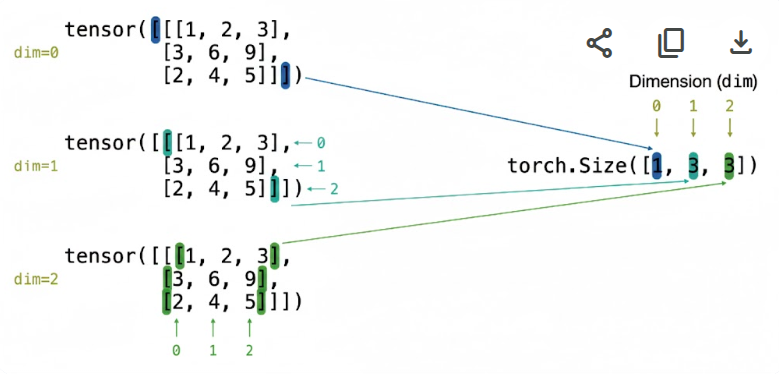
Understanding Tensor Shapes

distances = torch.tensor([[5.0], [6.0], [8.0], [10.0]])
distances.shape  # torch.Size([4, 1])

• First dimension: batch size (4 samples)
• Second dimension: features per sample (1 feature)

The shape tells you exactly how your data is organized. [4, 1] means 4 samples, each with 1 feature. This structure is crucial - PyTorch models expect input with a batch dimension. The first number tells the model how many samples it’s getting. The rest describe what each sample looks like.

If you had multiple features (distance, time of day, weather), each sample would have multiple values, but the batch structure would remain the same.

Tensor Dimensions: 3 dimensions

How to read brackets as dimensions

Creating the Model

model = nn.Sequential(
    nn.Linear(1, 1)  # 1 input, 1 output
)

Sequential: container that passes data through layers in order

Linear layer: single neuron (weight × input + bias)

Remember those rigid assembly lines from early deep learning frameworks? Sequential is PyTorch’s streamlined version. It’s a container that passes data through layers in order, but makes it easy for you to swap components without all that messy rewiring.

Here, you’re only using one layer - your single neuron. It’s technically a linear layer. The first 1 means it takes one input (distance). The second 1 means it produces one output (predicted delivery time). It applies a linear transformation to the input - that’s all the linear layer does.

This neuron will learn the best weight and bias to map distances to delivery times, just like finding the best-fitting line through all your data points.

Loss Function

loss_function = nn.MSELoss()

Mean Squared Error: measures how wrong predictions are

• Bigger errors → bigger loss
• Perfect predictions → loss = 0

Your model needs two tools to actually learn. The first is the loss function. We’re using Mean Squared Error loss, which measures how wrong or how right your predictions are.

If you predict 45 minutes when it actually took 60, that’s a bigger error than predicting 58 minutes. MSE captures this by squaring the differences, which makes bigger mistakes matter more. The goal is to minimize this loss - the lower the loss, the better your model.

Optimizer

optimizer = optim.SGD(model.parameters(), lr=0.01)

SGD (Stochastic Gradient Descent):

• Figures out which direction to adjust weights/bias
• lr (learning rate): controls step size

The optimizer is the algorithm that figures out which direction to adjust your weight and bias to reduce that error. model.parameters() is how you access those values in PyTorch - in this case, just the weight and bias from your single neuron.

lr is the learning rate. Smaller values mean you adjust parameters by smaller amounts. Larger values mean bigger adjustments. Both extremes can have challenges - too small and training is slow, too large and you might overshoot the best values.

If you’re curious about the math behind loss functions or optimization, you’ll get a much deeper introduction in Module 2.

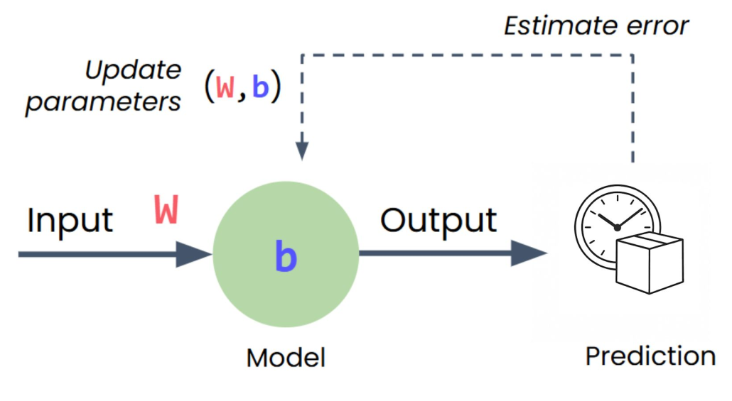
The Training Loop

for epoch in range(500):
    optimizer.zero_grad()      # Clear old calculations
    outputs = model(distances) # Make predictions
    loss = loss_function(outputs, times)  # Measure error
    loss.backward()            # Calculate gradients
    optimizer.step()           # Update weights/bias

Each epoch: one full pass through training data

This is the training loop where the actual learning happens. Remember when I manually adjusted the weight and bias to get closer to the right line? This code is doing the same thing automatically, hundreds of times.

Each full pass through the training data is called an epoch. In each epoch, the model will: (1) make predictions, (2) measure how far off those predictions are, and (3) adjust its internal parameters to improve.

Let’s break down each line: optimizer.zero_grad() clears out all calculated values from the previous training round. Without it, PyTorch would accumulate adjustments across rounds, which would mess up your learning.

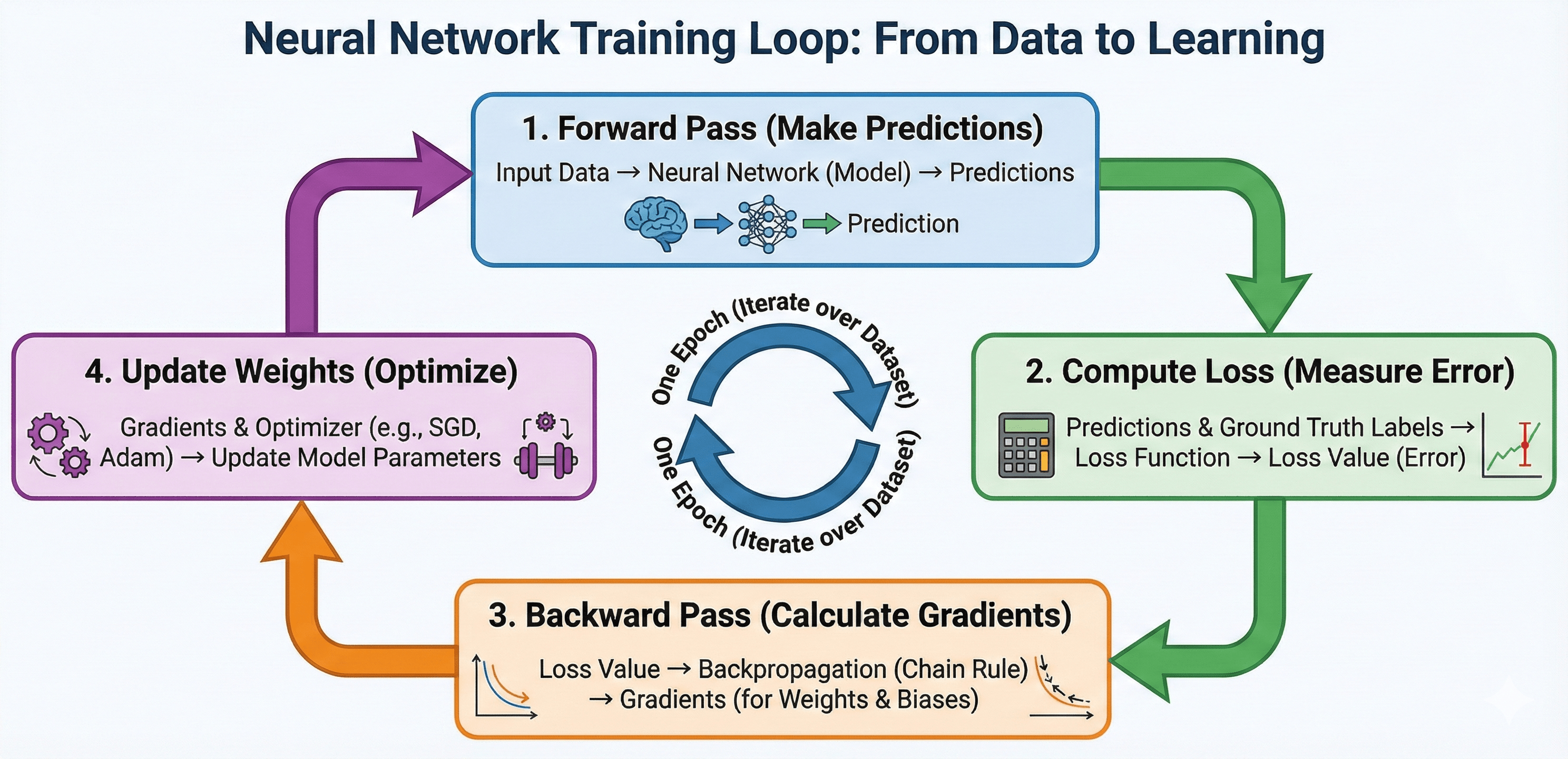
Training Loop Breakdown

outputs = model(distances) - Model uses distance as input

loss = loss_function(outputs, times) - Compares predictions to real times

loss.backward() - Figures out how to adjust weight/bias (backpropagation)

optimizer.step() - Makes the adjustments

outputs = model(distances) tells the model to use the distance as inputs and make predictions.

loss = loss_function(outputs, times) compares the predictions to the real times and calculates how wrong they are.

loss.backward() figures out how to adjust the weight and bias to reduce that error. Just like when I said “I need a steeper slope,” it’s now done with calculus behind the scenes. The technical term is backpropagation.

optimizer.step() makes all those adjustments. The model is now slightly better at predicting delivery times.

Making Predictions (Inference)

with torch.no_grad():
    new_distance = torch.tensor([[7.0]])
    prediction = model(new_distance)
    print(prediction)

torch.no_grad(): skip training overhead for faster inference

Now that the model is trained, let’s try making a prediction. The line with torch.no_grad() tells PyTorch that you’re not training anymore, just doing inference. Training takes extra work under the hood, but for inference, we can skip all that and run much more efficiently.

If the model learned what it was supposed to, it should give you a good answer. But you’re going to have to try it out in the lab to see for yourself.

Speaking of building, that’s exactly what’s next. It’s time to get hands-on and see if your delivery job is still safe.

Lab 1: Building a Simple Neural Network

“What I hear, I forget. What I see, I remember. What I do, I understand.”

START WITH LAB 1

What’s Next?

In Session 3: Activation Functions we learn:

• Why linear models fail for complex patterns
• Introducing non-linearity with activation functions
• ReLU and other activation functions

In the next session, we’ll discover what happens when your delivery company expands and the relationship between distance and time becomes non-linear. We’ll learn how activation functions help neural networks model curves and complex patterns, not just straight lines.