import seaborn as snsExercise: EDA on Penguins (Solution)
In this notebook tutorial, we will conduct simple EDA steps on the popular penguins dataset.
Load the dataset
Dataset source: https://www.kaggle.com/datasets/parulpandey/palmer-archipelago-antarctica-penguin-data
df = sns.load_dataset('penguins')
df.head()| species | island | bill_length_mm | bill_depth_mm | flipper_length_mm | body_mass_g | sex | |
|---|---|---|---|---|---|---|---|
| 0 | Adelie | Torgersen | 39.1 | 18.7 | 181.0 | 3750.0 | Male |
| 1 | Adelie | Torgersen | 39.5 | 17.4 | 186.0 | 3800.0 | Female |
| 2 | Adelie | Torgersen | 40.3 | 18.0 | 195.0 | 3250.0 | Female |
| 3 | Adelie | Torgersen | NaN | NaN | NaN | NaN | NaN |
| 4 | Adelie | Torgersen | 36.7 | 19.3 | 193.0 | 3450.0 | Female |
df.info()<class 'pandas.core.frame.DataFrame'>
RangeIndex: 344 entries, 0 to 343
Data columns (total 7 columns):
# Column Non-Null Count Dtype
--- ------ -------------- -----
0 species 344 non-null object
1 island 344 non-null object
2 bill_length_mm 342 non-null float64
3 bill_depth_mm 342 non-null float64
4 flipper_length_mm 342 non-null float64
5 body_mass_g 342 non-null float64
6 sex 333 non-null object
dtypes: float64(4), object(3)
memory usage: 18.9+ KBUnderstand the Features
Here is what I found on the internet from: https://www.kaggle.com/code/parulpandey/penguin-dataset-the-new-iris
species(categorical) is who the penguin belong to (Adelie, Chinstrap, Gentoo)island(categorical) is where the penguin came from (Biscoe, Dream, Torgersen)- bill (is the منقار) of the penguin, the thing which he uses to eat
bill_length_mm(numeric) in milimetersbill_depth_mm(numeric) in milimeter
- flipper are their wings
flipper_length_mm(numeric) in milimeter
sex(categorical) is the gender: Male or Femalebody_mass_g(numeric) in grams
Penguin Bill

Data Cleaning
Technical Dataframe Information
df.info()<class 'pandas.core.frame.DataFrame'>
RangeIndex: 344 entries, 0 to 343
Data columns (total 7 columns):
# Column Non-Null Count Dtype
--- ------ -------------- -----
0 species 344 non-null object
1 island 344 non-null object
2 bill_length_mm 342 non-null float64
3 bill_depth_mm 342 non-null float64
4 flipper_length_mm 342 non-null float64
5 body_mass_g 342 non-null float64
6 sex 333 non-null object
dtypes: float64(4), object(3)
memory usage: 18.9+ KB- missing values: We notice that there are some missing values in the dataset.
- categroical types:
species,island, andsexcan be converted tocategorydata type instead of the currentobjectdata type. - numerical types: To save memory,
bill_length_mm,bill_depth_mm,flipper_length_mm, andbody_mass_gcan be converted tofloat32instead offloat64.
We note that features are properly named and don’t need renaming or standardization.
Missing values
# count missing values
df.isnull().sum()
species 0
island 0
bill_length_mm 2
bill_depth_mm 2
flipper_length_mm 2
body_mass_g 2
sex 11
dtype: int64# percentage of missing values from each column
df.isnull().mean() * 100species 0.000000
island 0.000000
bill_length_mm 0.581395
bill_depth_mm 0.581395
flipper_length_mm 0.581395
body_mass_g 0.581395
sex 3.197674
dtype: float64Since missing values are low in number, we can safely drop them.
df.dropna(inplace=True)# optionally fill missing values with the mean
# df['bill_length_mm'].fillna(df['bill_length_mm'].mean(), inplace=True)Duplicates
Be sure to drop duplicates if any.
df.drop_duplicates(inplace=True)Data types conversion
- We shall convert the string types to
categoryto preserve memory - we shall also convert
float64 -> float32
mem_usage_before = df.memory_usage(deep=True)# convert categotical types
df['species'] = df['species'].astype('category')
df['island'] = df['island'].astype('category')
df['sex'] = df['sex'].astype('category')# convert numerical types
df['bill_depth_mm'] = df['bill_depth_mm'].astype('float32')
df['bill_length_mm'] = df['bill_length_mm'].astype('float32')
df['flipper_length_mm'] = df['flipper_length_mm'].astype('float32')
df['body_mass_g'] = df['body_mass_g'].astype('float32')mem_usage_after = df.memory_usage(deep=True)
print('memory saved:', (mem_usage_before - mem_usage_after).sum() // 1024, 'KB')memory saved: 64 KBDetect inconsistency in categorical values
The categorical columns should be checked for any inconsistencies. For example. We look for lowercase, uppercase, or inconsistent use of codes (e.g., “M”, “F”) with non-codes (e.g., “Male”, “Female”) in the sex column.
print(df['species'].unique())
print(df['island'].unique())
print(df['sex'].unique())
['Adelie', 'Chinstrap', 'Gentoo']
Categories (3, object): ['Adelie', 'Chinstrap', 'Gentoo']
['Torgersen', 'Biscoe', 'Dream']
Categories (3, object): ['Biscoe', 'Dream', 'Torgersen']
['Male', 'Female']
Categories (2, object): ['Female', 'Male']Summary data after cleaning
df.info()<class 'pandas.core.frame.DataFrame'>
Index: 333 entries, 0 to 343
Data columns (total 7 columns):
# Column Non-Null Count Dtype
--- ------ -------------- -----
0 species 333 non-null category
1 island 333 non-null category
2 bill_length_mm 333 non-null float32
3 bill_depth_mm 333 non-null float32
4 flipper_length_mm 333 non-null float32
5 body_mass_g 333 non-null float32
6 sex 333 non-null category
dtypes: category(3), float32(4)
memory usage: 9.2 KB(11 / 343) * 1003.206997084548105- After cleaning, the dataset was reduced from 343 to 333 rows, a difference of 10 rows
- The drop of sex na values resulted in a reduction of 3.2% of data size
- We imputed the missing numerical values with the mean
Dataset Size
df.shape(333, 7)Univariate Analysis
Distribution of categorical features
# categorical columns
df.describe(exclude='number').T| count | unique | top | freq | |
|---|---|---|---|---|
| species | 333 | 3 | Adelie | 146 |
| island | 333 | 3 | Biscoe | 163 |
| sex | 333 | 2 | Male | 168 |
species = df['species'].value_counts()
island = df['island'].value_counts()
sex = df['sex'].value_counts()
import matplotlib.pyplot as plt
fig, ax = plt.subplots(1, 3, figsize=(12, 5), sharey=True)
species.plot(kind='bar', ax=ax[0], color='skyblue', rot=0)
ax[0].set_title('Species')
ax[0].set_ylabel('Count')
ax[0].set_xlabel('Species')
island.plot(kind='bar', ax=ax[1], color='lightgreen', rot=0)
ax[1].set_title('Island')
ax[1].set_ylabel('Count')
ax[1].set_xlabel('Island')
sex.plot(kind='bar', ax=ax[2], color='salmon', rot=0)
ax[2].set_title('Sex')
ax[2].set_ylabel('Count')
ax[2].set_xlabel('Sex')Text(0.5, 0, 'Sex')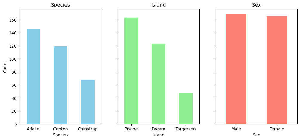
fig, ax = plt.subplots(1, 3, figsize=(12, 5))

species.plot(kind='pie', ax=ax[0], autopct='%1.1f%%', startangle=90, shadow=True)
ax[0].set_title('Species')
ax[0].set_ylabel('')

island.plot(kind='pie', ax=ax[1], autopct='%1.1f%%', startangle=90, shadow=True)
ax[1].set_title('Island')
ax[1].set_ylabel('')

sex.plot(kind='pie', ax=ax[2], autopct='%1.1f%%', startangle=90, shadow=True)
ax[2].set_title('Sex')
ax[2].set_ylabel('')

fig.show()
C:\Users\thund\AppData\Local\Temp\ipykernel_17424\1184769405.py:15: UserWarning: FigureCanvasAgg is non-interactive, and thus cannot be shown
fig.show()
Distribution of numerical features
# numerical columns
df.describe(include='number').T| count | mean | std | min | 25% | 50% | 75% | max | |
|---|---|---|---|---|---|---|---|---|
| bill_length_mm | 333.0 | 43.992794 | 5.468668 | 32.099998 | 39.5 | 44.500000 | 48.599998 | 59.599998 |
| bill_depth_mm | 333.0 | 17.164865 | 1.969235 | 13.100000 | 15.6 | 17.299999 | 18.700001 | 21.500000 |
| flipper_length_mm | 333.0 | 200.966965 | 14.015765 | 172.000000 | 190.0 | 197.000000 | 213.000000 | 231.000000 |
| body_mass_g | 333.0 | 4207.057129 | 805.215820 | 2700.000000 | 3550.0 | 4050.000000 | 4775.000000 | 6300.000000 |
import matplotlib.pyplot as plt

df_numeric = df.select_dtypes('number')

fig, axes = plt.subplots(nrows=2, ncols=2, figsize=(8, 4), gridspec_kw=dict(hspace=0.5, wspace=0.5))
fig.tight_layout() # Or equivalently,  "plt.tight_layout()"

for i, col in enumerate(df_numeric.columns):
    print(i, col)
    # df[col].plot.box(ax=axes.flat[i])
    df[col].plot.hist(ax=axes.flat[i])
    axes.flat[i].set_title(col)

plt.show()
C:\Users\thund\AppData\Local\Temp\ipykernel_17424\71577449.py:6: UserWarning: This figure includes Axes that are not compatible with tight_layout, so results might be incorrect.
fig.tight_layout() # Or equivalently, "plt.tight_layout()"0 bill_length_mm
1 bill_depth_mm
2 flipper_length_mm
3 body_mass_g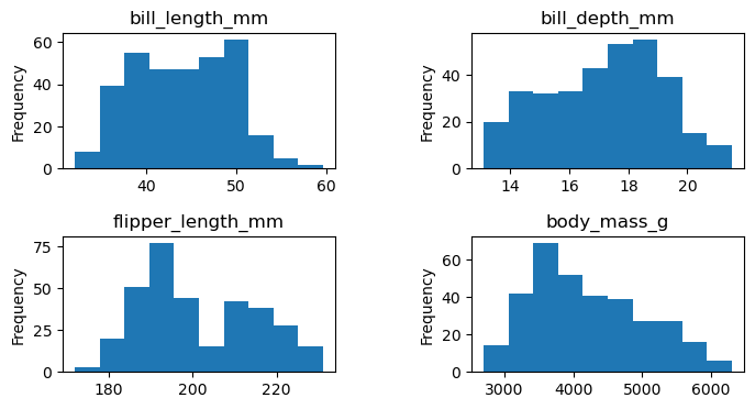
Bivariate Analysis
Correlation between numerical features
Let’s find out if there is any correlation between numerical features.
df.select_dtypes(include='number').corr()| bill_length_mm | bill_depth_mm | flipper_length_mm | body_mass_g | |
|---|---|---|---|---|
| bill_length_mm | 1.000000 | -0.228626 | 0.653096 | 0.589451 |
| bill_depth_mm | -0.228626 | 1.000000 | -0.577792 | -0.472016 |
| flipper_length_mm | 0.653096 | -0.577792 | 1.000000 | 0.872979 |
| body_mass_g | 0.589451 | -0.472016 | 0.872979 | 1.000000 |
numerical_corr = df.select_dtypes(include='number').corr()
sns.heatmap(numerical_corr, annot=True)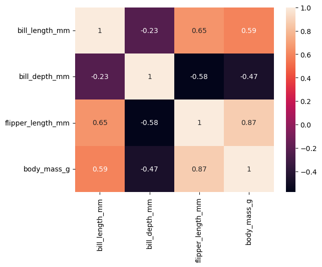
Observations:
- We notice high correlation between flipper length and body mass (0.87).
- We also notice high correlation between flipper length and bill length (0.65).
- There is little correlation between bill depth and bill length (-0.23).
sns.pairplot(df[['bill_length_mm', 'bill_depth_mm', 'species']])Looking at the previous scatter-plot showing "culmen length" and "culmen depth", the species are reasonably well separated:
- low culmen length -> Adelie
- low culmen depth -> Gentoo
- high culmen depth and high culmen length -> Chinstrap
There is some small overlap between the species, so we can expect a statistical model to perform well on this dataset but not perfectly.
Feature Engineering
- We might try adding the feature
bill_sizewhich is the product ofbill_lengthandbill_depthto see if it has any significance in the model. - We might also try
bill_ratiowhich is the ratio ofbill_lengthtobill_depthto see if it has any significance in the model.
df| species | island | bill_length_mm | bill_depth_mm | flipper_length_mm | body_mass_g | sex | |
|---|---|---|---|---|---|---|---|
| 0 | Adelie | Torgersen | 39.099998 | 18.700001 | 181.0 | 3750.0 | Male |
| 1 | Adelie | Torgersen | 39.500000 | 17.400000 | 186.0 | 3800.0 | Female |
| 2 | Adelie | Torgersen | 40.299999 | 18.000000 | 195.0 | 3250.0 | Female |
| 4 | Adelie | Torgersen | 36.700001 | 19.299999 | 193.0 | 3450.0 | Female |
| 5 | Adelie | Torgersen | 39.299999 | 20.600000 | 190.0 | 3650.0 | Male |
| ... | ... | ... | ... | ... | ... | ... | ... |
| 338 | Gentoo | Biscoe | 47.200001 | 13.700000 | 214.0 | 4925.0 | Female |
| 340 | Gentoo | Biscoe | 46.799999 | 14.300000 | 215.0 | 4850.0 | Female |
| 341 | Gentoo | Biscoe | 50.400002 | 15.700000 | 222.0 | 5750.0 | Male |
| 342 | Gentoo | Biscoe | 45.200001 | 14.800000 | 212.0 | 5200.0 | Female |
| 343 | Gentoo | Biscoe | 49.900002 | 16.100000 | 213.0 | 5400.0 | Male |
333 rows × 7 columns
df['bill_size'] = df['bill_length_mm'] * df['bill_depth_mm']
df['bill_ratio'] = df['bill_length_mm'] / df['bill_depth_mm']df.head()| species | island | bill_length_mm | bill_depth_mm | flipper_length_mm | body_mass_g | sex | bill_size | bill_ratio | |
|---|---|---|---|---|---|---|---|---|---|
| 0 | Adelie | Torgersen | 39.099998 | 18.700001 | 181.0 | 3750.0 | Male | 731.169983 | 2.090909 |
| 1 | Adelie | Torgersen | 39.500000 | 17.400000 | 186.0 | 3800.0 | Female | 687.299988 | 2.270115 |
| 2 | Adelie | Torgersen | 40.299999 | 18.000000 | 195.0 | 3250.0 | Female | 725.399963 | 2.238889 |
| 4 | Adelie | Torgersen | 36.700001 | 19.299999 | 193.0 | 3450.0 | Female | 708.309998 | 1.901554 |
| 5 | Adelie | Torgersen | 39.299999 | 20.600000 | 190.0 | 3650.0 | Male | 809.580017 | 1.907767 |
corr = df.corr(numeric_only=True)corr['body_mass_g'].sort_values().plot.barh()
sns.heatmap(df.corr(numeric_only=True), annot=True)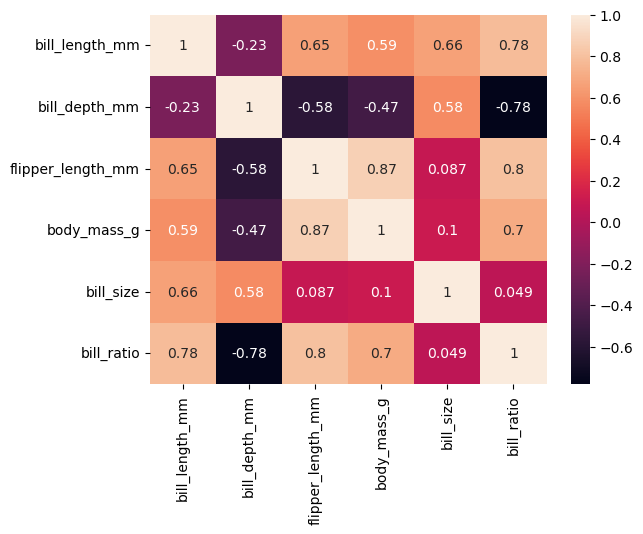
Extra
Hypothesize and test
We think that penguins may differ in terms of body mass between species, as well as by gender.
A boxplot can be used to verify this hypothesis.
sns.boxplot(data=df, x='species', y='body_mass_g', hue='sex')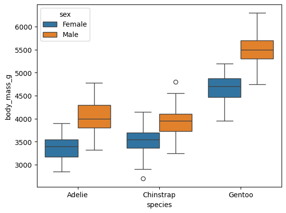
Observations:
- Our assumption seems correct (at least visually); i.e., Gentoo penguins are heavier than Adélie and Chinstrap penguins.
- We were also right about females’ weight. Females are lighter across all species!
sns.displot(df, kind='kde', x='body_mass_g', hue='sex', col='species', fill=True)
sns.swarmplot(df, y='body_mass_g', x='species', hue='sex')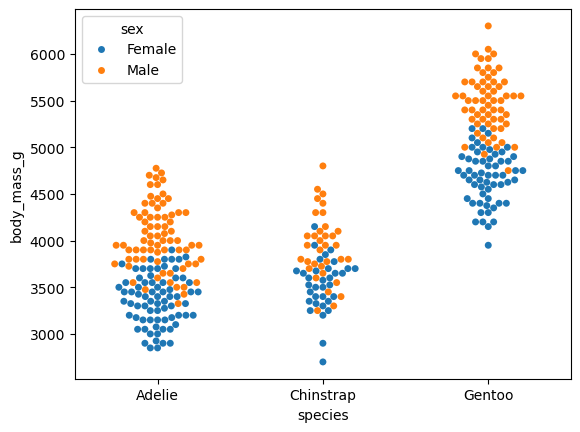
Categorical and Categorical
import pandas as pd

cross = pd.crosstab(df['island'], df['species'], normalize=True)
cross| species | Adelie | Chinstrap | Gentoo |
|---|---|---|---|
| island | |||
| Biscoe | 0.132132 | 0.000000 | 0.357357 |
| Dream | 0.165165 | 0.204204 | 0.000000 |
| Torgersen | 0.141141 | 0.000000 | 0.000000 |
sns.heatmap(cross, annot=True)<Axes: xlabel='species', ylabel='island'>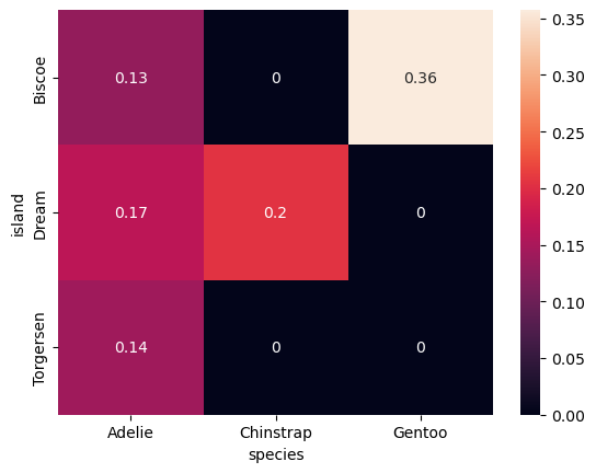
- We can use a heatmap with correlation matrix (numerical vs numerical)
- values range between (-1 and +1)
- We used a heatmap here with contigency matrix (categorical vs categorical)
- values in the entire table sum up to one
- range is (0 to 1)
# plot numerical columns
sns.pairplot(df, hue='species')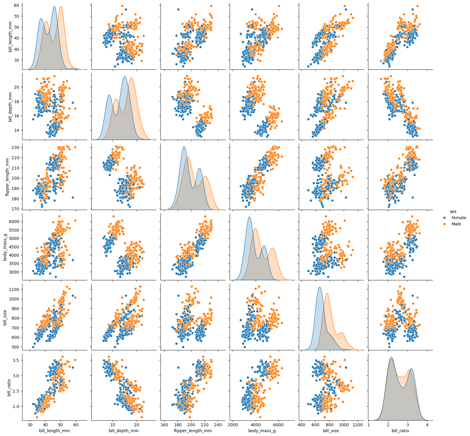
- Distribution plots can tell us a lot about each species.
- Scatter plots can tell us about the relationship between features.